The Timed LBO Modeling Test: Full Tutorial for a 60-Minute Case Study

The LBO modeling test, just like the private equity case study, is one of the scariest parts of the recruiting process for many candidates.

But it’s a bit misleading to call it a “modeling test.”

Given the time constraints – often between 1 and 3 hours – it’s more of an Excel speed test.

If you know the shortcuts and formulas like the back of your hand, and you can enter data quickly, you should do quite well.

And if not, you better start learning and practicing ASAP.

We’ll go through a full practice run in this tutorial for a 60-minute test starting from a blank sheet:

Types of LBO Modeling Tests

As discussed in the PE case study article, there are different types of “modeling tests” and “case studies”: simple paper LBOs, 1-3-hour timed tests, and open-ended take-home case studies.

The 1-3-hour timed tests are most common in the on-cycle recruiting process at large firms in the U.S.

However, they could come up in any recruiting process; for example, some firms in London start with a simple, timed test to screen candidates before advancing them to the next rounds.

The good news is that these timed tests require far less critical thinking, creativity, and research than the open-ended case studies.

The bad news is that if you want to get good at them, you’ll need to “put in the reps” by completing many practice exercises.

What to Expect in a Timed LBO Modeling Test

The two main categories are tests that give you an Excel template and tests in which you start from a blank sheet.

The ones with templates tend to have more complex formulas, and the ones where you start from scratch have simpler formulas but are more challenging to finish under time pressure.

Here’s a summary of the likely differences based on the type and allotted time:

The 60-Minute LBO Modeling Test from a Blank Sheet

You can find examples of tests with provided templates fairly easily, so I thought it would be more interesting to look at an example without a template here.

You can get the case study prompt, the answers, and the completed Excel file below:

• 60-Minute LBO Modeling Test – Case Study Prompt (PDF)
• 60-Minute LBO Modeling Test – Completed Excel File (XL)
• Answers to Case Study Questions (PDF)
• Overview of Main Points in 60-Minute LBO Modeling Test – Slides (PDF)

There is no “blank” or “beginning” file because we create a new sheet in Excel and enter everything from scratch in this tutorial.

You can get the video version of this entire tutorial below:

Table of Contents:

• 2:24: Part 1: Likely Requirements in Modeling Tests
• 7:43: Part 2: Transaction Assumptions and Sources & Uses
• 17:24: Part 3: Model Drivers and Income Statement
• 32:14: Part 4: Free Cash Flow and Debt Schedule
• 46:04: Part 5: Returns and Sensitivities
• 56:22: Part 6: Answers to the Case Study Questions
• 1:03:12: Recap and Summary

This example is not taken from our courses – it’s new for this article – but it is similar to one of the many case studies in our Core Financial Modeling course:

Core Financial Modeling

Learn accounting, 3-statement modeling, valuation/DCF analysis, M&A and merger models, and LBOs and leveraged buyout models with 10+ global case studies.

learn more

The full course has a different 60-minute example and a 90-minute test as well. And if you want more complex LBO models and a “take-home” example, check out the Advanced Financial Modeling course:

Advanced Financial Modeling

Learn more complex "on the job" investment banking models and complete private equity, hedge fund, and credit case studies to win buy-side job offers.

learn more

Part 1: Likely Requirements in an LBO Modeling Test

The chart above sums up the likely requirements for tests of different lengths. To be more specific, you can expect the following in a 60-minute test starting from a blank sheet:

• Assumptions: Purchase Enterprise Value or Equity Value and a simple Sources & Uses schedule. There may be a working capital adjustment as well, but it’s fairly simple and makes a low impact on the model.
• Debt Schedule: Perhaps 2-3 tranches of Debt with slightly different interest rates and repayment terms (e.g., fixed vs. floating interest, cash vs. PIK, and mandatory and optional repayments for one tranche). A Revolver is possible but unlikely.
• Revenue, Expenses, and Cash Flow: These will often be simple percentage assumptions, but they could be a bit more complicated, such as Units Sold * Average Unit Price or Market Share * Market Size.
• Financial Statements: A simple Income Statement and partial Cash Flow Statement; you just need enough to calculate Free Cash Flow and Cash Flow Available for Debt Repayment.
• Returns Calculations: These will be fairly simple, but there could be a small twist, such as an earn-out, options pool, or management rollover.
• Sensitivity Analysis: You might create 1-2 tables if the returns calculations were simple, but you might skip these if they were more complex. The case study questions determine whether or not you “need” these tables.
• Total # of Rows: Probably ~100 or less (including blank rows), but you could go up to ~130 if there are sensitivities.

Unless they specifically ask you to do so, you should NOT build a full 3-statement model.

It’s a waste of time when you have only 60 minutes and adds nothing over the cash flow projections.

You should also skip other bells and whistles such as purchase price allocation, scenarios, complex Debt schedules, etc.

And do not include anything beyond bare-bones formatting, or you’ll never finish on time – number formats are OK, but forget about colors and borders for headers, input boxes, etc.

Part 2: Transaction Assumptions and Sources & Uses

The first part of this exercise is simple: we enter the assumptions provided in the case study document, focusing on ones that stay the same each year:

Since this is a cash-free, debt-free deal, we use Purchase Enterprise Value on the Uses side of the Sources & Uses schedule.

One slightly tricky part is the $25 million “Cash Injection” when the deal closes; the case document strongly hints that we need to include this:

“Cash-free, debt-free” means the company has 0 Cash and 0 Debt immediately after the deal closes – but that changes a second later due to the new Debt used to fund the deal.

There isn’t always a “Cash injection” right after the deal closes, but in this case, there is.

The rest is straightforward, and the Investor Equity is a standard “plug,” as shown above (Total Uses – Sources So Far).

Part 3: Model Drivers and Income Statement

It helps to start by setting up a sketch of the Income Statement, so we know what we’re building up to:

Then, we can go back and fill in some of the drivers, starting with widget unit sales and the average price per widget:

The document gives us information about the factories, including Maintenance CapEx and Growth CapEx, but it’s vague about the Depreciation.

You might be tempted to do something complicated, such as a detailed Depreciation schedule based on annual CapEx spending.

Or you might want to use functions like ROUNDUP to ensure that the factory count can only be in whole units rather than decimals (“8.5 factories” doesn’t make logical sense).

I recommend avoiding all of this and keeping the drivers as simple as possible because these details do not matter in a time-pressured test.

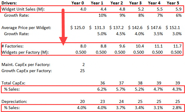
We drive the # of factories with the Widget Unit Sales and the Widgets per Factory, which is 500,000 based on the initial year (4 million widgets / 8 factories).

Depreciation is a simple % of sales, set to percentages slightly below the CapEx ones:

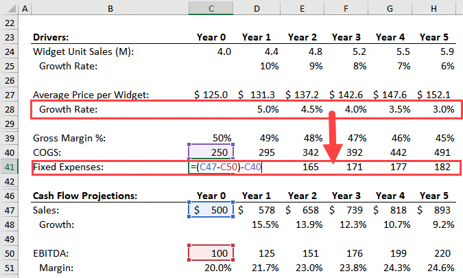
The COGS and Operating Expenses ( “Fixed Expenses” here) are simple; COGS is based on the Gross Margin %, and Fixed Expenses = (Sales – EBITDA) – COGS.

They grow at the same rate as average widget pricing:

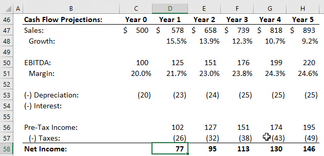
We can then put together all the pieces to build the Income Statement down to Net Income, skipping the Interest deduction for now:

Part 4: Free Cash Flow and Debt Schedule

Free Cash Flow, at least under U.S. GAAP, is defined as Cash Flow from Operations minus CapEx (roughly).

“Cash Flow from Operations” is simple because this company is simple: start with Net Income, add Depreciation and Non-Cash Interest, and add/subtract the Change in Working Capital.

And then subtract Total CapEx from the model drivers to calculate FCF:

To complete the blank lines here, we need the Interest numbers – but to get the Interest expense, we need the Debt balances first.

But before we can project the Debt balances, we need to think about optional repayments, otherwise known as “cash flow sweeps.”

In other words, if the company generates positive cash flow available for Debt repayment in one year, how much of that cash flow could it use to repay the Term Loans optionally?

The case document explicitly tells us the answer is “50%”:

However, it’s NOT as simple as using 50% of the “Free Cash Flow” to repay these Term Loans.

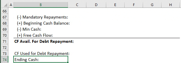
“Cash Flow Available for Debt Repayment” is different from “Free Cash Flow” because more line items factor into it:

• FCF Generated in the Year: This increases the cash the company could potentially use to repay the Term Loans.
• Beginning Cash: The higher the company’s initial Cash balance, the more it can potentially use to repay Debt.
• Mandatory Repayments: If the company must repay 5%, 10%, or 15% of the Term Loans, these payments reduce how much it can pay optionally.
• Minimum Cash: Finally, Widget Co. must maintain 5% of its previous year’s sales as a minimum Cash balance at all times, which reduces the amount it can use to repay Debt.

Putting these pieces together, we get this sketch:

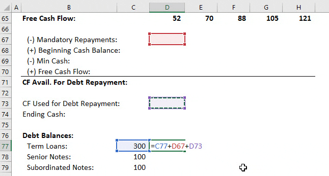
At this stage, we should move to the Debt balances below and link the Term Loans to the mandatory and optional repayments and the Senior and Subordinated Notes to PIK Interest:

And then, we can go back and calculate the Cash Flow Used for Debt Repayment and the Ending Cash each year:

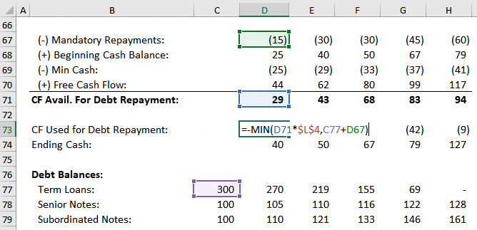
NOTE: In the video, the Ending Cash calculation is incorrect at first. We go back and fix it a few minutes later. The screenshot above reflects the correct numbers at this stage of the model.

The Cash Flow Used for Debt Repayment is the minimum between the Cash Flow Available * Sweep % and the remaining Term Loan balance after the mandatory repayment.

This formula ensures that if, for example, $50 of the Term Loan remains, but we have $200 * 50% = $100 in available cash flow, only the remaining $50 is repaid.

The Ending Cash is based on the Beginning Cash minus Mandatory Debt Repayments plus Free Cash Flow minus Optional Repayments (“CF Used for Debt Repayment”).

The final step is to calculate the interest for each tranche of Debt, which we split into Cash and PIK to make it easier to link the statements later:

We then go back and link the total Interest Expense into the Income Statement and add back the Paid-in-Kind portions to calculate Free Cash Flow:

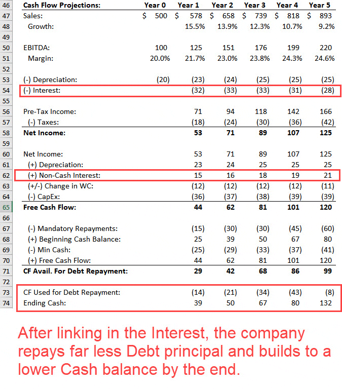
As a result of these Interest links, the company’s Cash balance grows to a lower level, and it repays the Term Loans more slowly.

To avoid circular references, we can use the beginning Debt balance as well (for more, see our tutorial on how to remove circular references in Excel).

Part 5: Returns and Sensitivities

The basic returns calculations here are simple: we apply an Exit Multiple to the EBITDA in Year 4 or 5 to calculate the Exit Enterprise Value, subtract the remaining Debt, and add the remaining Cash:

The 5% management options pool makes things trickier, as we need to factor in the Cash the management team pays to exercise their options and the Equity they receive.

By paying to exercise their options, the management team increases the total Equity, which means they no longer own exactly 5% of the total Equity.

Management owns 5% / (1 + 5%) = ~4.8% of this expanded pool, so the Equity to Management Option Holders is based on that percentage times the expanded total Equity:

If you get this slightly wrong, it’s not the end of the world; this point barely affects the returns.

You just need to show some small outflow of proceeds, assuming the Exit Equity Value is higher than the initial Investor Equity (meaning the options are exercisable).

We can then calculate the IRR and multiple of invested capital and create a few simple sensitivity tables:

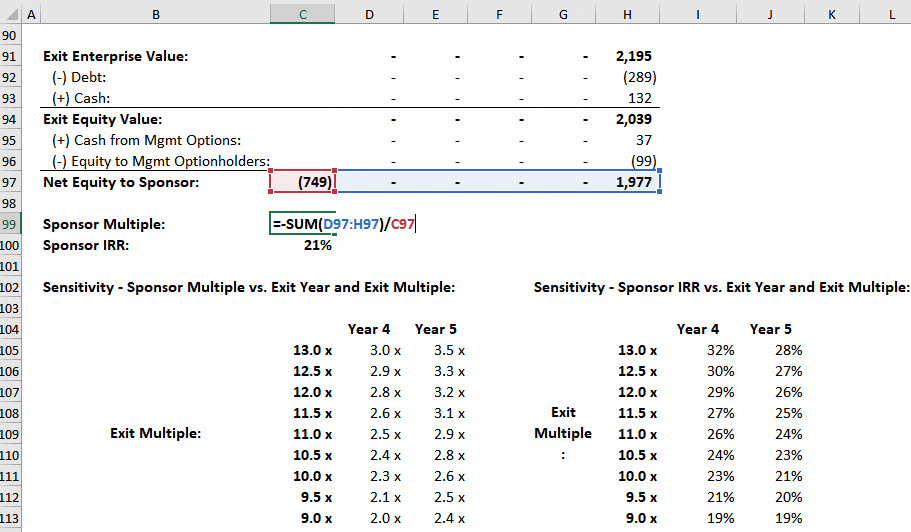
If you’re wondering about the exit multiple range of 9-13x, the purchase multiple was 12x, and the company is growing more slowly by the end of the holding period (~9% vs. ~16%), so we assumed modestly lower multiples.

Ideally, we’d look at the ROIC and comparable companies to estimate the exit multiple, but we do not have the time or information for those.

With that, we’re done with the Excel portion of this modeling test.

Part 6: Answers to the Case Study Questions

You can read the answers yourself, but in short, we recommend doing this deal because the likely IRRs are between 20% and 30%, with MOICs between 2x and 3x.

The company’s financial projections may be slightly aggressive in terms of margin expansion (with EBITDA margins increasing from 20% to 25%), but growth is also slowing, so they’re not crazy.

If the PE firm wants to boost its returns, the easiest solution is to use more Debt.

The company can support more than 5x Debt / EBITDA because it pays off the Term Loans by Year 5, with Total Debt falling by over $200 million in that period.

So, the PE firm could increase the initial Debt to 6x or do a Dividend Recap midway through the holding period (or even a simple cash dividend).

How to Master the LBO Modeling Test

Overall, this is a fairly challenging LBO modeling test.

I intentionally inserted multiple ways to make mistakes and waste time on marginally useful tasks.

That said, you do not need to score 100% to “pass” – the median score on these tests is often below 50%.

So, if you can finish the model and get most of it correct, you should be in good shape, even with some mistakes here and there.

But the key part of that sentence is “finish the model.”

If you don’t know Excel quite well, you will struggle to finish in 60 minutes.

If it takes you 2-3 hours to finish, that’s a fine result for your first try.

At that level, you could reduce your time to the 60-minute range with repeated practice.

Similar to standardized tests like the SAT and GMAT, there are only so many features they could throw at you in an LBO modeling test.

Once you’ve done 5-10 practice tests, you’ll be ready for ~90% of future tests.

And if the average person suddenly learned the truth about what it takes to get into private equity, they might start wondering what explains those sky-high salaries…